05: Circuit Simulation
In the previous part of this tutorial we built a simple digital circuit simulator using several application kernels running on multiple SpiNNaker chips which communicated with multicast packets. In our proof-of-concept host program, the chip and core to use for each kernel was chosen by hand and all routing tables were written manually. Though this works, it made our simulator incredibly inflexible and the host program hard to modify and extend.
In this part of the tutorial we’ll leave the application kernels unchanged but re-write our host program to make use of the automatic place-and-route tools provided by Rig. These tools automate the process of assigning application kernels to specific cores and generating routing tables while attempting to make efficient use of the machine. We’ll also restructure our host program to be more like a real-world application complete with a simple user-facing interface.
The source files used in this tutorial can be downloaded below:
- Host program
- Example circuit simulation script
- SpiNNaker kernels (unchanged from part 04)
Defining the circuit simulator user interface/API
If our circuit simulator is to be useful it must present a sensible API to allow users to describe their circuits. In this example we’ll implement an API which looks like this:
import sys

from circuit_simulator import Simulator, Stimulus, Or, And, Probe

# Define a 64 ms simulation to be run on the given SpiNNaker machine
sim = Simulator(sys.argv[1], 64)

# Define three stimulus generators which together produce all 8 combinations of
# values.
stimulus_a = Stimulus(
    sim, "0000000011111111000000001111111100000000111111110000000011111111")
stimulus_b = Stimulus(
    sim, "0000000000000000111111111111111100000000000000001111111111111111")
stimulus_c = Stimulus(
    sim, "0000000000000000000000000000000011111111111111111111111111111111")

# Define the two gates
or_gate = Or(sim)
and_gate = And(sim)

# Define a probe to record the output of the circuit
probe = Probe(sim)

# Wire everything together
or_gate.connect_input("a", stimulus_a.output)
or_gate.connect_input("b", stimulus_b.output)

and_gate.connect_input("a", stimulus_c.output)
and_gate.connect_input("b", or_gate.output)

probe.connect_input(and_gate.output)

# Run the simulation
sim.run()

# Print the results
print("Stimulus A: " + stimulus_a.stimulus)
print("Stimulus B: " + stimulus_b.stimulus)
print("Stimulus C: " + stimulus_c.stimulus)
print("Probe:      " + probe.recorded_data)
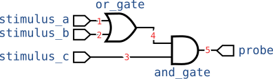
This script defines the same circuit which we hard-coded in part 04:
With our desired API in mind, lets design our circuit simulator!
Place and Route using Rig
Before diving into the code it is first important to understand what the Rig place-and-route tools do.
Rig provides a suite of placement and routing algorithms in its
rig.place_and_route module. In essence, these algorithms accept
abstract descriptions of graphs of communicating SpiNNaker application kernels
as input. Based on this information the place and route algorithms select which
core each kernel will be loaded onto, keeping communicating cores close
together to reduce network load. In addition, routing tables which make
efficient use of SpiNNaker’s network are generated.
In Rig terminology, the abstract (hyper-)graph of application kernels are known as vertices which are connected together by nets:
- vertices
- Approximately speaking, a vertex represents a group of cores and SDRAM which must be assigned in one piece to a chip somewhere. In our circuit simulator, a vertex represents a single gate, stimulus or probe and each requires a single core and some quantity of SDRAM.
- nets
- A net typically represents a 1-to-many flow of multicast packets between vertices. A net has a single source vertex and many sink vertices. In our circuit simulator, a net corresponds to a wire in our circuit, where the source is the gate or stimulus output driving the wire and the sinks are the connected gate and probe inputs.
In addition to graph of vertices and nets, the place and route tools require a
description of the SpiNNaker machine our simulation will be running on. As we
will see later, the MachineController provides
a method for gathering this information.
Building the circuit simulator API
What follows is a (non-linear) walk-through of the most important parts of the
circuit simulator host program provided in circuit_simulator.py.
In most host applications built with Rig, the graph of vertices and nets fed to the place and route tools are generated from application-specific data structures shortly before performing the place-and-route. This allows the majority of the application to use data structures which best fit the application. In this circuit simulator example we’ll follow this approach too, so let’s start by defining the Python classes which make up the API.
Defining a wire
A wire represents a connection from one the output of one component to the inputs of many other components and is defined as follows:
class _Wire(object):
    """A wire which connects one component's output to many components'
    inputs.

    For internal use: to be constructed via :py:meth:`.Simulator._new_wire`
    only.
    """

    def __init__(self, source, sinks, routing_key):
        """Defines a new wire from source to sinks which will use the specified
        routing key.

        Parameters
        ----------
        source : component
        sinks : [component, ...]
        routing_key : int
        """
        self.source = source
        self.sinks = sinks
        self.routing_key = routing_key
A _Wire instance contains a source component, a list of sink
components and a unique routing key to use in the simulation. The Simulator
object (to be defined later) will be responsible for creating new _Wire
objects.
Defining components (gates, stimuli and probes)
At the heart of our circuit simulator is our two-input, one-output,
lookup-table-based logic gate so let’s define our Gate component first like
so:
class Gate(object):
    """A 2-input 1-output logic gate implemented using a lookup-table."""

    def __init__(self, simulator, lookup_table):
        """Define a new gate.

        Parameters
        ----------
        simulator : :py:class:`.Simulator`
            The simulator which will be responsible for simulating this gate.
        lookup_table : int
            A lookup table giving the output value of the gate as a 4-bit
            number where each bit gives the output for a particular combination
            of input values.

            =======  =======  ==============
            input a  input b  lut bit number
            =======  =======  ==============
            0        0        0
            1        0        1
            0        1        2
            1        1        3
            =======  =======  ==============
        """
        self._simulator = simulator
        self._lookup_table = lookup_table

        # Register this component with the simulator
        self._simulator._add_component(self)

        # The two inputs, initially not connected
        self._inputs = {"a": None, "b": None}

        # A new wire will be created and sourced by this gate
        self.output = self._simulator._new_wire(self)

    def connect_input(self, name, wire):
        """Connect the specified input to a wire."""
        self._inputs[name] = wire
        wire.sinks.append(self)
In the constructor we simply store a reference to the Simulator object
along with a copy of the lookup table provided. We also inform the
Simulator of the existance of the component using
Simulator._add_component. The _inputs attribute will hold references to
the _Wires connected to each input and the output attribute holds a
reference to (a newly created) _Wire which will be driven by the gate.
The Gate.connect_input method connects a _Wire to an input by storing a
reference to the _Wire object and adding the component to the _Wire’s
list of sinks.
We also define various subclasses of Gate which, for the sake of
convenience, simply define the lookup table to be used. For example an AND-gate
component is defined like so:
class And(Gate):
    """An AND gate."""

    def __init__(self, simulator):
        super(And, self).__init__(simulator, 0b1000)
The Probe object is defined in a similar way to the Gate but doesn’t
define an output:
class Probe(object):
    """A 1-bit recording probe."""

    def __init__(self, simulator):
        """Define a new probe.

        Parameters
        ----------
        simulator : :py:class:`.Simulator`
            The simulator in which the probe will be used.
        """
        self._simulator = simulator
        self.recorded_data = None

        # Register this component with the simulator
        self._simulator._add_component(self)

        # The input, initially disconnected
        self._input = None

    def connect_input(self, wire):
        """Probe the specified wire."""
        self._input = wire
        wire.sinks.append(self)
Finally, the Stimulus object is defined but, since it doesn’t have any
inputs, the connect_input method is excluded:
class Stimulus(object):
    """A 1-bit stimulus source."""

    def __init__(self, simulator, stimulus=""):
        """Define a new stimulus source.

        Parameters
        ----------
        simulator : :py:class:`.Simulator`
            The simulator in which the stimulus will be used.
        stimulus : str
            A string of "0" and "1"s giving the stimulus to generate for each
            millisecond in the simulation. Will be zero-padded or truncated to
            match the length of the simulation.
        """
        self._simulator = simulator
        self.stimulus = stimulus

        # Register this component with the simulator
        self._simulator._add_component(self)

        # A new wire will be created sourced by this stimulus generator
        self.output = self._simulator._new_wire(self)
Defining the simulator
All that remains to be defined of our API is the Simulator object. The
Simulator simply stores the hostname and simulation length provided and
maintains lists of components and wires which have been added to the
simulation:
class Simulator(object):
    """A SpiNNaker-based digital logic simulator."""

    def __init__(self, hostname, length):
        """Create a new simulation.

        Parameters
        ----------
        hostname : str
            The hostname or IP of the SpiNNaker machine to use.
        length : int
            The number of milliseconds to run the simulation for.
        """
        self._hostname = hostname
        self.length = length

        # A list of components added to the simulation
        self._components = []

        # A list of wires used in the simulation
        self._wires = []

    def _add_component(self, component):
        """Add a component to the simulation.

        Called internally by components on construction.
        """
        self._components.append(component)

    def _new_wire(self, source, sinks=None):
        """Create a new :py:class:`._Wire` with a unique routing key."""
        # Assign sequential routing key to new nets.
        wire = _Wire(source, sinks if sinks is not None else [], len(self._wires))
        self._wires.append(wire)

        return wire
Making it work
At this point, our API is complete with the notable exception of the
Simulation.run() method. At a high level, the run() method performs
the following steps:
- Build a graph of the form accepted by Rig’s place and route tools.
- Perform place and route.
- Load the configuration data, routing tables and application kernels required.
- Run the simulation.
- Read back results captured by probes.
We’ll now proceed to break down this function and look at its operation in detail.
Building a place-and-routeable graph
To perform place and route we must build a graph describing our simulation in the format required by Rig.
The first thing we need to do is define the resources required by each vertex
in the graph. Rig allows us to use any Python object to represent a
vertex and since each component in our simulation will become a vertex in our
graph we’ll use the objects we defined above to identify the
vertices. We build a vertices_resources dictionary which enumerates the
resources consumed by each vertex in our application:
vertices_resources = {
    # Every component runs on exactly one core and consumes a certain
    # amount of SDRAM to hold configuration data.
    component: {Cores: 1, SDRAM: component._get_config_size()}
    for component in self._components
}
Each entry in the vertices_resources dictionary contains another dictionary
mapping ‘resources’ to the required quantities of each resource. As in most
applications, the only resources we care about are Cores and SDRAM. By
convention these resources are identified to by the corresponding
Cores and SDRAM
sentinels defined by Rig.
Each vertex requires exactly one core but the amount of SDRAM required depends
on the type of component and length of the simulation. A _get_config_size()
method is added to each of our component types to compute their SDRAM
requirements:
class Gate(object):
    def _get_config_size(self):
        """Get the size of configuration block needed for this gate."""
        # The config contains 5x uint32_t
        return 5 * 4
class Probe(object):
    def _get_config_size(self):
        """Get the size of configuration block needed for this probe."""
        # The config contains 2x uint32_t and a byte for every 8 bits of
        # recorded data.
        return (2 * 4) + ((self._simulator.length + 7) // 8)
class Stimulus(object):
    def _get_config_size(self):
        """Get the size of configuration block needed for this stimulus."""
        # The config contains 2x uint32_t and a byte for every 8 bits of
        # stimulus data.
        return (2 * 4) + ((self._simulator.length + 7) // 8)
Next we must also define the filename of the spinnaker application kernel (i.e. the APLX file) used for each vertex.
vertices_applications = {component: component._get_kernel()
                         for component in self._components}
Once again we support this by adding a _get_kernel() method to each
component type:
class Gate(object):
    def _get_kernel(self):
        """Get the filename of the SpiNNaker application kernel to use."""
        return "gate.aplx"
class Probe(object):
    def _get_kernel(self):
        """Get the filename of the SpiNNaker application kernel to use."""
        return "probe.aplx"
class Stimulus(object):
    def _get_kernel(self):
        """Get the filename of the SpiNNaker application kernel to use."""
        return "stimulus.aplx"
Next, we enumerate the nets representing the streams of multicast packets
flowing between vertices, as well as the routing keys and masks used for each
net. Rig expects nets to be defined by Net objects.
Like the _Wire objects in our simulator, Nets
simply contain a source vertex and a list of sink vertices. In the code below
we build a dict mapping Nets to (key,
mask) tuples for each wire in the simulation:
net_keys = {Net(wire.source, wire.sinks): (wire.routing_key,
                                           0xFFFFFFFF)
            for wire in self._wires}
nets = list(net_keys)
The final piece of information required is a description of the SpiNNaker
machine onto which our application will be placed and routed. Using a
MachineController we first
boot() the machine and then
interrogate it using
get_system_info() which returns
a SystemInfo object. This
object contains a detailed description of the machine, for example, enumerating
working cores and links. This description will be used shortly to perform place
and route.
mc = MachineController(self._hostname)
mc.boot()
system_info = mc.get_system_info()
Place and route
The place and route process can be broken up into many steps such as placement,
allocation, routing and routing table generation. Though some advanced
applications may find it useful to break these steps apart, our circuit
simulator, like many other applications, does not. Rig provides a
place_and_route_wrapper() function which saves us
from the ‘boilerplate’ of doing each step separately. This function takes the
graph description we constructed above and performs the place and route process
in its entirety.
placements, allocations, application_map, routing_tables = \
    place_and_route_wrapper(vertices_resources,
                            vertices_applications,
                            nets, net_keys,
                            system_info)
The placements and allocations dict returned by
place_and_route_wrapper() together define the
specific chip and core each vertex has been assigned to (see
place() and
allocate() for details).
application_map is a dict describing what application kernels
need to be loaded onto what cores in the machine.
Finally, routing_tables contains a dict giving the routing
tables to be loaded onto each core in the machine.
Loading and running the simulation
We are now ready to load and execute our circuit simulation on SpiNNaker. The first step is to allocate blocks of SDRAM containing configuration data on every chip where our application kernels will run.
The sdram_alloc_for_vertices() utility
function takes a MachineController and the
placements and allocations dicts produced during place
and route and allocates a block of SDRAM for each vertex. Each allocation is
given a tag matching the core number of the vertex, and the size of the
allocation is determined by the quantity of
SDRAM consumed by the vertex, as originally
indicated in vertices_resources.
memory_allocations = sdram_alloc_for_vertices(mc, placements,
                                              allocations)
The dict returned is a mapping from each vertex (i.e. instances of
our component classes) to a
MemoryIO file-like
interface to SpiNNaker’s memory.
We add a _write_config method to each of our component classes which is
passed a MemoryIO object
into which configuration data is written.
for component, memory in memory_allocations.items():
    component._write_config(memory)
The _write_config functions for each component type are as follows:
class Gate(object):
    def _write_config(self, memory):
        """Write the configuration for this gate to memory."""
        memory.seek(0)
        memory.write(struct.pack("<5I",
                                 # sim_length
                                 self._simulator.length,
                                 # input_a_key
                                 self._inputs["a"].routing_key
                                 if self._inputs["a"] is not None
                                 else 0xFFFFFFFF,
                                 # input_b_key
                                 self._inputs["b"].routing_key
                                 if self._inputs["b"] is not None
                                 else 0xFFFFFFFF,
                                 # output_key
                                 self.output.routing_key,
                                 # lut
                                 self._lookup_table))
class Probe(object):
    def _write_config(self, memory):
        """Write the configuration for this probe to memory."""
        memory.seek(0)
        memory.write(struct.pack("<II",
                                 # sim_length
                                 self._simulator.length,
                                 # input_key
                                 self._input.routing_key
                                 if self._input is not None
                                 else 0xFFFFFFFF))
class Stimulus(object):
    def _write_config(self, memory):
        """Write the configuration for this stimulus to memory."""
        memory.seek(0)
        memory.write(struct.pack("<II",
                                 # sim_length
                                 self._simulator.length,
                                 # output_key
                                 self.output.routing_key))

        # NB: memory.write will automatically truncate any excess stimulus
        memory.write(bitarray(
            self.stimulus.ljust(self._simulator.length, "0"),
            endian="little").tobytes())
Next, the routing tables and SpiNNaker applications are loaded using
load_routing_tables() and
load_application():
# Load all routing tables
mc.load_routing_tables(routing_tables)

# Load all SpiNNaker application kernels
mc.load_application(application_map)
We now wait for the applications to reach their initial barrier, send the ‘sync0’ signal to start simulation and, finally, wait for the cores to exit.
# Wait for all six cores to reach the 'sync0' barrier
mc.wait_for_cores_to_reach_state("sync0", len(self._components))

# Send the 'sync0' signal to start execution and wait for the
# simulation to finish.
mc.send_signal("sync0")
time.sleep(self.length * 0.001)
mc.wait_for_cores_to_reach_state("exit", len(self._components))
The last step is to read back results from the machine. As with loading, we add
a _read_results method to each component type which we call with a
MemoryIO object from which
it should read any results it requires:
for component, memory in memory_allocations.items():
    component._read_results(memory)
The _read_results method is a no-op for all but the Probe component
whose implementation is as follows:
class Probe(object):
    def _read_results(self, memory):
        """Read back the probed results.

        Returns
        -------
        str
            A string of "0"s and "1"s, one for each millisecond of simulation.
        """
        # Seek to the simulation data and read it all back
        memory.seek(8)
        bits = bitarray(endian="little")
        bits.frombytes(memory.read())
        self.recorded_data = bits.to01()
Trying it out
Congratulations! Our circuit simulator is now complete! We can now run the example script we used to define our simulator’s API and within a second or so we have our results!
$ python example_circuit.py HOSTNAME_OR_IP
Stimulus A: 0000000011111111000000001111111100000000111111110000000011111111
Stimulus B: 0000000000000000111111111111111100000000000000001111111111111111
Stimulus C: 0000000000000000000000000000000011111111111111111111111111111111
Probe:      0000000000000000000000000000000001000000001111111111111111111111